
To receive Masat-1, the location and timing of it’s appearance must be known. The location and timing is not easy to determine, as the satellite is a 10 cm cube orbiting 300-1400 km from the Earth’s surface. The task is the following: to determine the orbit of our satellite. The task is simplified by the fact that we only have to choose from 9 objects corresponding to the spacecraft ejected to this orbit. The selection was made based on radio frequency Doppler-shift.
The process was the following: For each object, the variation of the signal’s apparent receive frequency at the observation point was determined based on the published TLEs using AGI STK 9. For each satellite, the different radial velocity and position gives a different variation of the apparent frequency based on Doppler effect. The SW calculated the trajectories from the TLEs using SGP4 algorithm. The apparent frequency was measured during radio contacts at satellite passes. The measured and calculated data were depicted on a common figure, according to which a decision was made.
To ease the measurements, a specific TLE had been chosen from the initial 9. The corresponding dynamic frequency shift was programmed to the radio by a PC and manual fine-tuning was applied. In every case, the resulting frequency (base+shift+tune) was recorded. The antenna was pointed to the proper direction with a proprietary software running on a PC, based on the same TLE as the one used for the calculation of the apparent frequency.
First we noted the frequency by hand with a 30 sec. sampling interval. The timing of this method was inaccurate due to the possibility of human error. To improve time-domain accuracy, manual recording was replaced by computer-based data recording. A sampling interval of 1 sec was used with a Yaesu FT897D radio and proprietary software. The apparent frequency was tracked based on the frequency waterfall of the signal. The frequencies were held within a window of 100 Hz. As the distance between the satellites increased, the graphs of time-frequency functions shifted away, making it apparent which object is Masat-1.
The two major sources of error are the deviation of the satellite’s transmitter from the nominal frequency (with which the calculations were made) and the imprecision of the time base used for the measurement. The transmit frequency of Masat-1 may deviate from the nominal 437.345 MHz, as the base oscillator shows some temperature dependence. Furthermore, the actual CW carrier frequency is 1.2 KHz upwards from the nominal, at 437.3462 MHz, to enable the USB reception of the transmitted GFSK signal at 437.345 MHz. In our case, this 1.2 kHz difference is added to the nominal receive frequency, with an error margin of less than 0.1 Hz. We neglected relativistic effects, which account for an error of 1 Hz. To reduce the error coming from the time base imprecision, the measurement computer was set to synchronize it’s clock with the time.windows.com internet-based time reference daily, giving an approximate time base error of 1 sec. A further error source is the inaccuracy of TLEs, as the SW calculated the trajectories based on them.
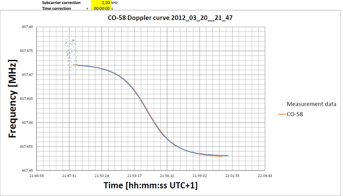
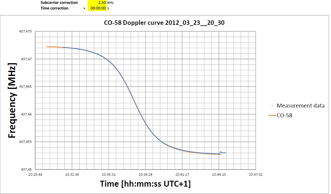
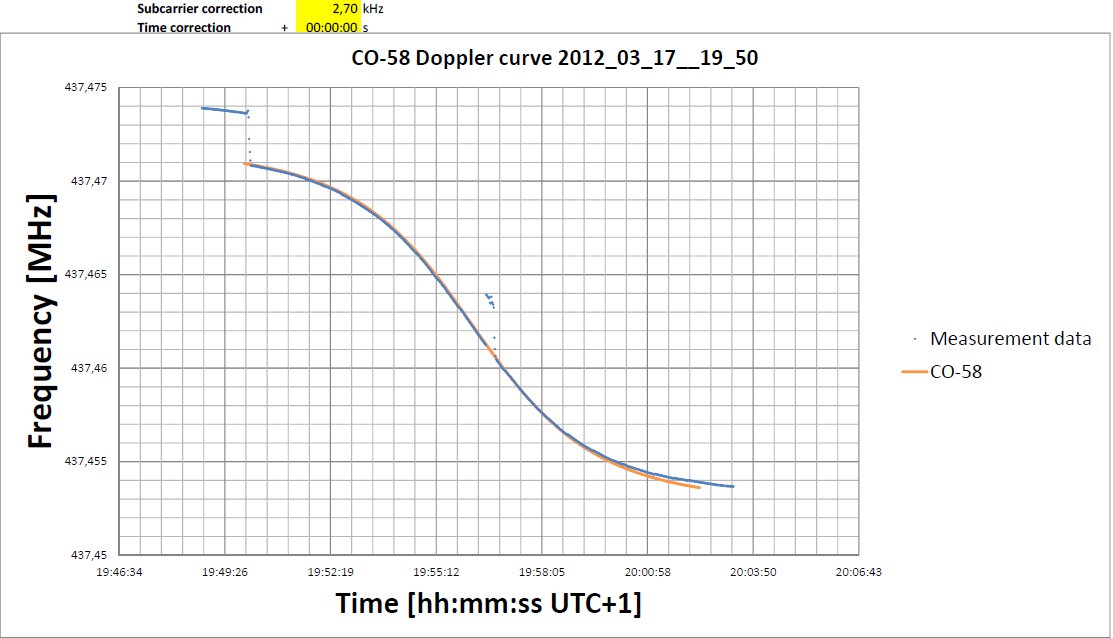
To verify the accuracy of our measurements, we carried out the same measurements and corresponding calculations with another satellite, CO-58. This is a Japanese satellite, launched in 2003, which, since 2003, have been transmitting with CW at the nominal frequency of 437.465 MHz, from which it deviates with +1.2 kHz, according to measurements.
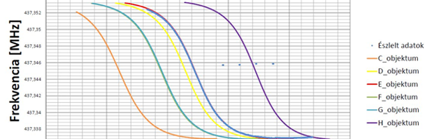
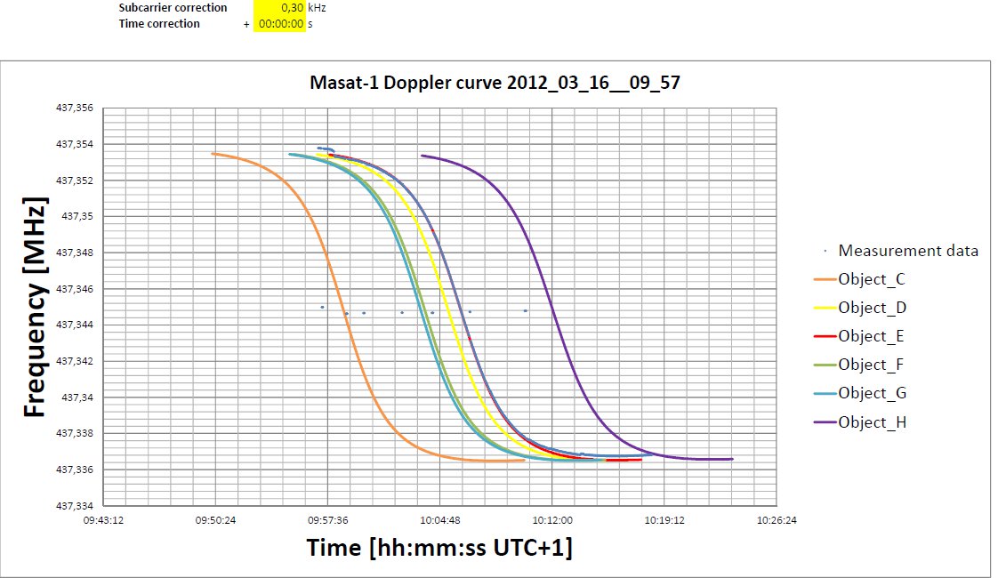
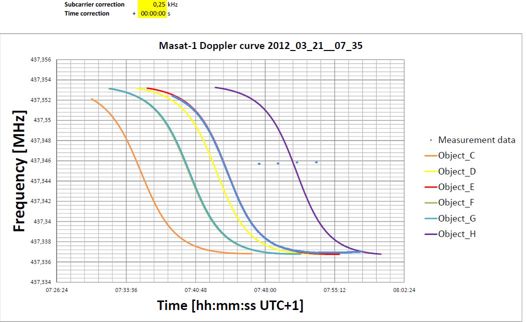
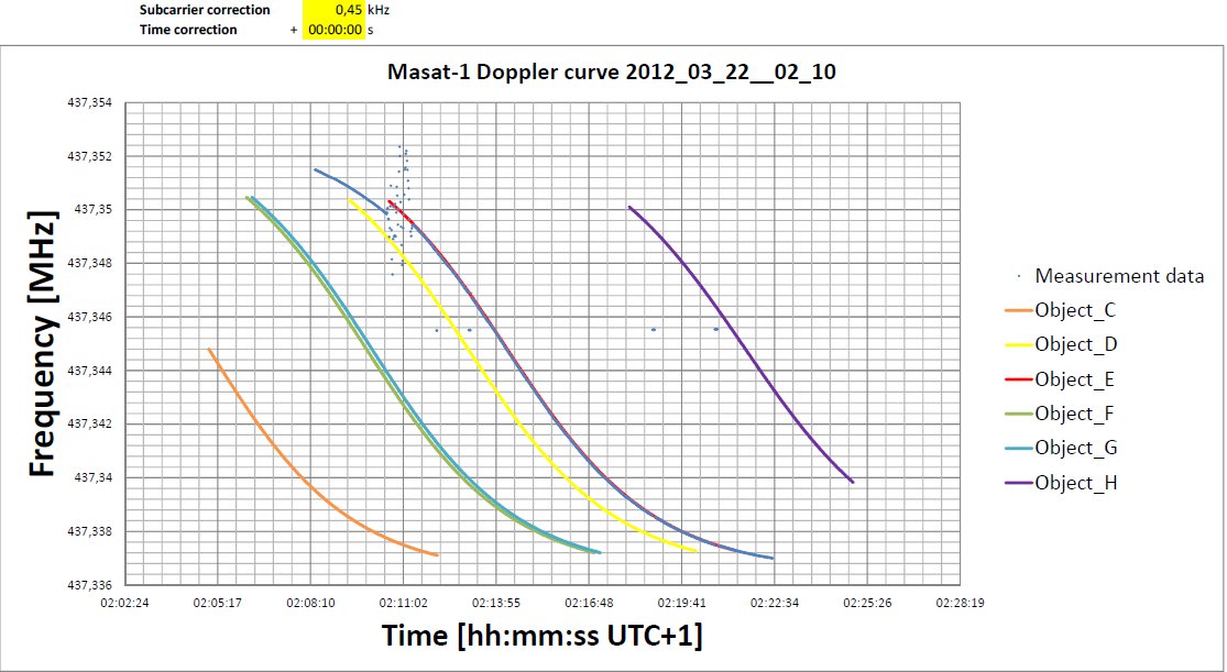
The results of the measurements and the corresponding calculations can be seen on the figures below. The horizontal axis is the time in CET winter time (UTC+1 hour), with hours-minutes-seconds. The vertical axis is the radio frequency in MHz. The noted subcarrier correction and time correction gives the shift of the calculated data in the horizontal and vertical axis compared to the measurement data to have the best fit of the two curves. With this data, the transmitted frequency and the absolute time measurement error can be corrected. On the curve corresponding to Masat-1, the regular erroneous points come from the transmit periods of the receiving station (GND TX turned on to command the satellite). At the beginning of the curves, one can observe scattered, erroneous values, this is when the tracking of the satellite was not yet locked.
In summary, it can be verified that the error between the measurement data and the calculated curves shows a minimum in case of object E, and a significantly higher value in case of the data of other objects. From the reference measurements carried out with CO-58 it can be well observed, that the known frequency error of the transmitter, being in the range of 1-2 kHz, can be corrected well, giving matching curves. A decisive fact is that even without the correction of the time base, the observed and calculated curves differ with less than 1-2 seconds at the section where the frequency change is the most significant. With this, the matching of the absolute time reference and the time reference calculated from the TLEs can also be verified.
The magnitude of difference is the same in case of the data of Masat-1 and object E. Object D is nearest to object E, but the time and frequency distance of it, being 20-60 seconds in the time domain, 1000-2000 Hz in the frequency domain, are much greater than the measurement error. Therefore the two objects can be explicitly distinguished based on Doppler measurements.
In conclusion, it can be stated with a high probability that Masat-1 is object E.